Getting Started
This is a simple example of the basic capabilities of aneris.
First, model and history data are read in. The model is then harmonized. Finally, output is analyzed.
[1]:
import pandas as pd
import seaborn as sns
import matplotlib.pyplot as plt

import aneris
from aneris.tutorial import load_data

%matplotlib inline
The driver is used to execute the harmonization. It will handle the data formatting needed to execute the harmonizaiton operation and stores the harmonized results until they are needed.
Some logging output is provided. It can be suppressed with
aneris.logger().setLevel('WARN')
[2]:
model, hist, driver = load_data()
for scenario in driver.scenarios():
    driver.harmonize(scenario)
harmonized, metadata, diagnostics = driver.harmonized_results()
INFO:root:Downselecting prefix|suffix variables
INFO:root:Translating to standard format
c:\users\gidden\work_tmp\aneris\aneris\utils.py:634: FutureWarning: In a future version, `df.iloc[:, i] = newvals` will attempt to set the values inplace instead of always setting a new array. To retain the old behavior, use either `df[df.columns[i]] = newvals` or, if columns are non-unique, `df.isetitem(i, newvals)`
  df.loc[where, numcols(df)] *= 1e3
INFO:root:Aggregating historical values to native regions
INFO:root:Harmonizing (with example methods):
INFO:root:                                              method            default  \
region  gas sector
regionc BC  prefix|sector1|suffix  reduce_ratio_2100  reduce_ratio_2050
            prefix|sector2|suffix  reduce_ratio_2050  reduce_ratio_2050
            prefix|suffix          reduce_ratio_2050  reduce_ratio_2050

                                            override
region  gas sector
regionc BC  prefix|sector1|suffix  reduce_ratio_2100
            prefix|sector2|suffix                NaN
            prefix|suffix                        NaN
INFO:root:and override methods:
INFO:root:region   sector                 gas
regionc  prefix|sector1|suffix  BC     reduce_ratio_2100
Name: method, dtype: object
INFO:root:Harmonizing with reduce_ratio_2100
INFO:root:Harmonizing with reduce_ratio_2050
WARNING:root:Removing sector aggregates. Recalculating with harmonized totals.
c:\users\gidden\work_tmp\aneris\aneris\utils.py:447: FutureWarning: The default value of numeric_only in DataFrameGroupBy.sum is deprecated. In a future version, numeric_only will default to False. Either specify numeric_only or select only columns which should be valid for the function.
  rows = self.df.groupby(grp_idx).sum().reset_index()
INFO:root:Translating to IAMC template
BAZ
region   sector                 gas
regionc  prefix|sector1|suffix  BC     reduce_ratio_2100
Name: method, dtype: object
BAZZ
                                              method            default  \
region  gas sector
regionc BC  prefix|sector1|suffix  reduce_ratio_2100  reduce_ratio_2050
            prefix|sector2|suffix  reduce_ratio_2050  reduce_ratio_2050
            prefix|suffix          reduce_ratio_2050  reduce_ratio_2050

                                            override
region  gas sector
regionc BC  prefix|sector1|suffix  reduce_ratio_2100
            prefix|sector2|suffix                NaN
            prefix|suffix                        NaN
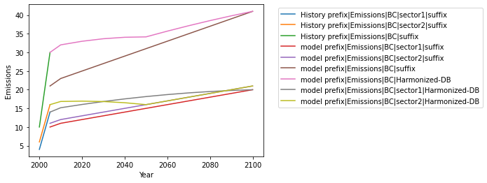
All data of interest is combined in order to easily view it. We will specifically investigate output for the World in this example. A few operations are performed in order to get the data into a plotting-friendly format.
[3]:
data = pd.concat([hist, model, harmonized])
df = data[data.Region.isin(['World'])]
[4]:
df = pd.melt(df, id_vars=aneris.iamc_idx, value_vars=aneris.numcols(df),
             var_name='Year', value_name='Emissions')
df['Label'] = df['Model'] + ' ' + df['Variable']
[5]:
df.head()
[5]:
| Model | Scenario | Region | Variable | Year | Emissions | Label | |
|---|---|---|---|---|---|---|---|
| 0 | History | scen | World | prefix|Emissions|BC|sector1|suffix | 2000 | 4.0 | History prefix|Emissions|BC|sector1|suffix |
| 1 | History | scen | World | prefix|Emissions|BC|sector2|suffix | 2000 | 6.0 | History prefix|Emissions|BC|sector2|suffix |
| 2 | History | scen | World | prefix|Emissions|BC|suffix | 2000 | 10.0 | History prefix|Emissions|BC|suffix |
| 3 | model | sspn | World | prefix|Emissions|BC|sector1|suffix | 2000 | NaN | model prefix|Emissions|BC|sector1|suffix |
| 4 | model | sspn | World | prefix|Emissions|BC|sector2|suffix | 2000 | NaN | model prefix|Emissions|BC|sector2|suffix |
[6]:
sns.lineplot(x=df.Year.astype(int), y=df.Emissions, hue=df.Label)
plt.legend(bbox_to_anchor=(1.05, 1))
[6]:
<matplotlib.legend.Legend at 0x1c5ad0428e0>